In 5 easy steps to your first deep learning model

With fast.ai everyone can train their own deep learning model. Only 5 steps are necessary.

1. Find a dataset
2. Make data available in code
3. Prepare data
4. Training of the model
5. Use it

We want to train a neural network to help doctors detect pneumonia from x-rays. We will go through the process step by step. The learning success is best if you type the lines yourself.

1. Find a dataset

Without data there is no machine learning - that is clear. Since we want to classify image data in this example, there are several ways to get a data set. - You already have data. In the example if you are a radiologists. - Collect images from the internet ("scrapping") - Use public data sets

In this case, we use the last approach because it is easy and available to everyone. Known data sets are MINST (handwritten numbers), .... Large picture DB or ... A place to found a range of datasets is Kaggle. On this platform, competitions on machine learning topics take place. The data sets are also public, because everybody can participate in the competitions. There we find our x-ray images, which are already "labeled". This means that this images are classified as normal or sick. After downloading the data we are ready for the next step.

2. Make data available in code

Python is used as programming language. As intuitive programming environment we use Jupiter notebook. You can use Google Colab or Paperspace for free to start. I can recommend the last one. Here we use fast.ai library, because there are many functions already available to run own models quickly. YOu can run all code snippets in a new cell.

from fastai import *

After importing the library, we check whether the directory with the training data is located in the right place. If not already done, the downloaded folder has to be unzipped and moved into the folder with the Jupiter notebook.

!ls

We can now see that the folder is in the right place. After that we set the path to the images and check a second time if everything worked out fine.

Path.BASE_PATH = Path('./chest_xray_data/')
path = Path.BASE_PATH
Path.BASE_PATH.ls()

3. Prepare data

Because we process images. Let's first check if there are files in the image folder that are not images and could later lead to errors.

fns = get_image_files(path)
fns

Next, we crate a DataBlock which contains information about our data and for the train process later.

xrays = DataBlock(
    # indicates that our input data are images and our predictions are categories
    blocks=(ImageBlock, CategoryBlock),
    # specifies the input data as images from the provided path
    get_items=get_image_files,
    # splitting the dataset in train and validationset randomy with seed 42
    splitter=RandomSplitter(valid_pct=0.2, seed=42),
    # sets the label as the name of the partent directory
    get_y=parent_label,
    # resizes images to 128px x 128px
    item_tfms=Resize(128)
)

4. Training

Surprisingly, most of the work is inside the preparation. After the structure of the network has been defined (Datablock) and linked to the training data (Dataloader), we are ready.

dls = xrays.dataloaders(path)

Now, we can watch in the preperad data by looking at the first four pictures from the first batch.

dls.valid.show_batch(max_n=4, nrows=1)

Output:

Next, we train the convolutional neural network (CNN), a special type of neural network that is particularly suitable for image data. In addition, we use a pre-trained model ("Resnet18") to get better resultes quickly and set the target metric to the error rate in the validation set.

learn = cnn_learner(dls, resnet18, metrics=error_rate)

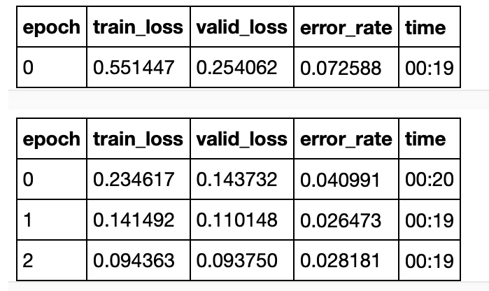
The learning process takes longer or shorter depending on the computer. After the first run, however, the model already reaches over 90% accuracy. The error rate can be further reduced by more training

learn.fine_tune(2)

Output

In this example, an accuracy of over 97% is achieved.

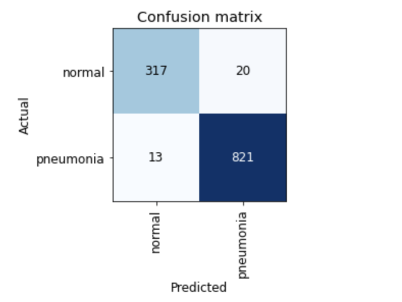
A more precise evaluation provides 13 false negative and 20 false positive of a total of 1171 images

interp = ClassificationInterpretation.from_learner(learn)
interp.plot_confusion_matrix()

Output:

The top 5 images where the model is most uncertain can be viewed above this command and any incorrectly forked data can be identified.

interp.plot_top_losses(5, nrows=1)

Finally, we can save the model for later use without training again.

learn.export()

5. Apply

We can import the saved model

learn_inf = load_learner("./export.pkl")

and use the neural network to predict a new image.

pred, pred_idx, probs = learn_inf.predict(img)
result = f"Predictions: {pred}; Probability: {probs[pred_idx]:.04f}"
result

Bonus

This snippet creates a widget to upload a imgage which is than classified.

from ipywidgets import VBox
btn_upload = widgets.FileUpload()
out_pl = widgets.Output()
lbl_pred = widgets.Label()
btn_run = widgets.Button(description="Classify")

def on_click_classify(change):
    img = PILImage.create(btn_upload.data[-1])

    out_pl.clear_output()
    with out_pl: display(img.to_thumb(128, 128))

    #get predictions
    pred, pred_idx, probs = learn_inf.predict(img)


    lbl_pred.value = f"Predictions: {pred}; Probability: {probs[pred_idx]:.04f}"
    lbl_pred

btn_run.on_click(on_click_classify)
VBox([widgets.Label("Select Image"), btn_upload, btn_run, out_pl, lbl_pred])
result

Now, we are done and have a simple classifier to support dotors!

See the repo here on GitHub.